Case Study One: Social behaviour during a badger lifetime
Matthew Silk
2020-07-03
CaseStudyOne.RmdExample of using CMRnet to generate movement networks of European badgers for use in analyses linking deaths caused by collisions with cars to the position of groups within movement networks
Background
This case study is based on a long-term CMR dataset from a high-density population of European badgers in the United Kingdom (Delahay et al., 2013; McDonald, Robertson, & Silk, 2018). Badgers in medium to high-density populations live in territorial social groups centred on a main sett (refuge/burrow system), resulting in modular social networks in which they interact frequently with other group members but much less often with individuals from other groups (Weber et al., 2013). The study population is trap-sampled four times per year (in May-June, July-August, September-October and December-January) using baited cage traps deployed at all know active sett locations (see McDonald et al., 2018 for more detail). Badgers give birth in late-winter (the date of birth of all cubs is assumed to be 1st February) and no trapping takes place while females have dependent cubs.
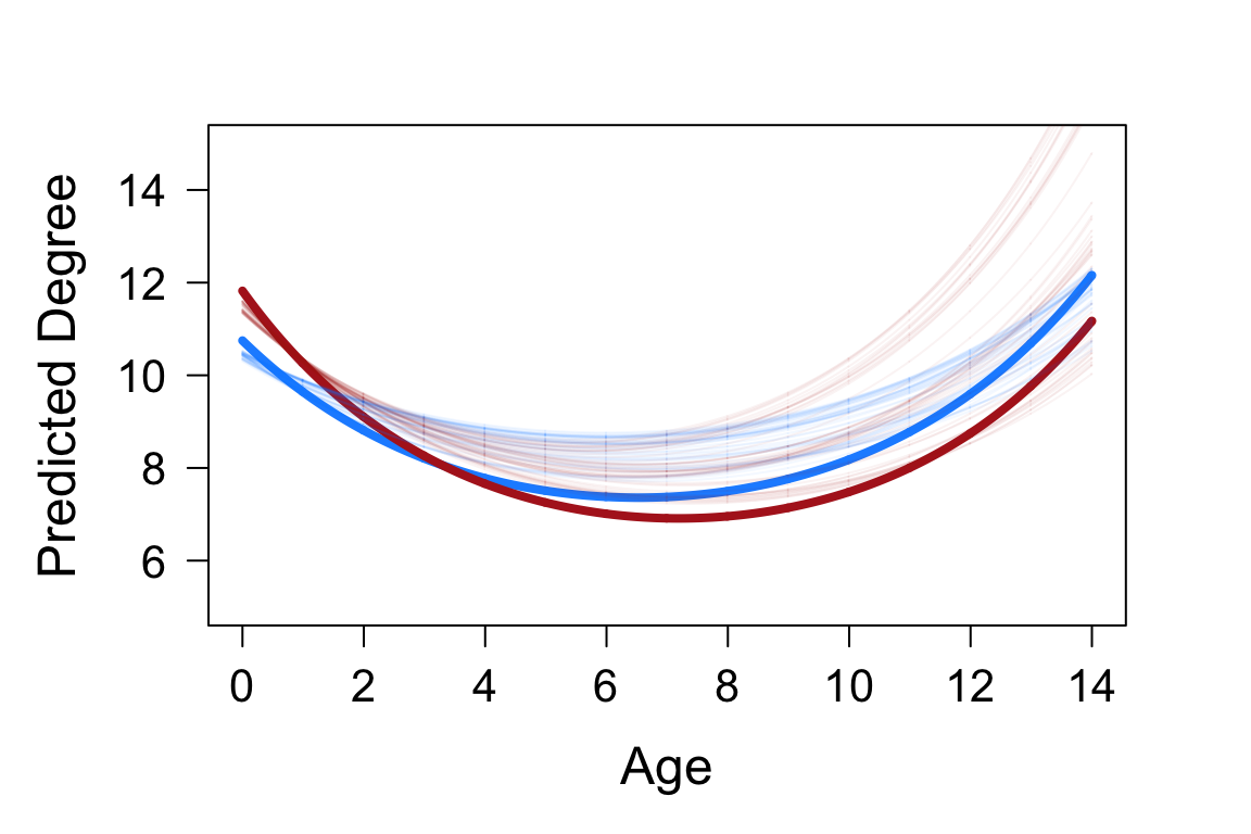
Here we use the co-capture network construction features of CMRnet to examine how the social network position of badgers changes during their lifetime. Individuals that are more strongly connected to those in other groups will be more central to the population network. We expect that the centrality of individuals in social networks peaks when levels of reproductive behaviour as this drives many between-group movements and interactions. Badgers in our study population demonstrate body mass and immune senescence, and so we would expect network centrality to peak in early adulthood, subsequent to maturity but prior to condition beginning to decline. We would also predict that this peak will be higher in males than females, due to differences in social and spatial behaviour.
Setup and data manipulation
First we set up our environment.
The data we use here is not documented in the package, but can be accessed to recreate this analyses by using CMRnet:::capturesData and CMRnet:::individualData.
# look at dimensions of data
str(captures)
#> 'data.frame':    14461 obs. of  6 variables:
#>  $ tattoo     : chr  "Y001" "Y002" "G020" "B031" ...
#>  $ date       : chr  "10/06/1981" "10/06/1981" "11/06/1981" "12/06/1981" ...
#>  $ socg       : chr  "WEST" "SEPTIC TANK" "SEPTIC TANK" "SEPTIC TANK" ...
#>  $ sett       : chr  "WEST" "SEPTIC TANK" "SEPTIC TANK" "SEPTIC TANK" ...
#>  $ CaptureYear: int  1981 1981 1981 1981 1981 1981 1981 1981 1981 1981 ...
#>  $ where      : chr  "SETT" "SETT" "SETT" "SETT" ...
str(indivdat)
#> 'data.frame':    2975 obs. of  4 variables:
#>  $ tattoo : chr  "001A" "001B" "001E" "001F" ...
#>  $ age_fc : chr  "CUB" "ADULT" "CUB" "ADULT" ...
#>  $ year_fc: int  2014 2006 2013 2010 2003 2012 2011 2009 2008 2004 ...
#>  $ sex    : chr  "FEMALE" "MALE" "FEMALE" "MALE" ...
We then do some data manipulation to fill in data on the age and sex of badgers in the captures data set. We also wrangle the date formats and create a dataframe in the format needed for CMRnet.
# create empty columns for sex and age
captures$sex<-rep(NA,nrow(captures))
captures$age<-rep("ADULT",nrow(captures))

# fill in data on the age and sex of badgers in the captures dataset
for(i in 1:nrow(captures)){
  if(captures$tattoo[i]%in%indivdat$tattoo){
    captures$sex[i]<-as.character(indivdat$sex[indivdat$tattoo==as.character(captures$tattoo[i])])
    if(substr(captures$date[i],7,10)==indivdat$year_fc[indivdat$tattoo==as.character(captures$tattoo[i])]&(is.na(indivdat$age_fc[indivdat$tattoo==as.character(captures$tattoo[i])])==FALSE)&indivdat$age_fc[indivdat$tattoo==as.character(captures$tattoo[i])]=="CUB"){
      captures$age[i]<-"CUB"
    }
    if(substr(captures$date[i],7,10)==indivdat$year_fc[indivdat$tattoo==as.character(captures$tattoo[i])]&(is.na(indivdat$age_fc[indivdat$tattoo==as.character(captures$tattoo[i])])==TRUE)){
      captures$age[i]<-NA
    }
  }
}

# Convert sex to a factor
captures$sex <- as.factor(captures$sex)

# Add a date column in correct format
captures$date2 <- as.Date(paste0(substr(captures$date,7,10),"-",substr(captures$date,4,5),"-",substr(captures$date,1,2)))

# Add year, month and day columns
captures$year <- lubridate::year(captures$date2)
captures$month <- lubridate::month(captures$date2)
captures$day <- lubridate::day(captures$date2)

# Create a year of study column
captures$year_of_study <- rep(NA,nrow(captures))
for(i in 1:nrow(captures)){
  if(captures$month[i]>1){
    captures$year_of_study[i]<-as.numeric(captures$year[i])-1985
  }
  if(captures$month[i]==1){
    captures$year_of_study[i]<-as.numeric(captures$year[i])-1986
  }
}

# Subset data to only include 30 years - Feb 1986 to Jan 2016
captures2 <- captures[captures$year_of_study>0&captures$year_of_study<31,]

# Create a dataframe in the correct format for CMRnet
captures3<-data.frame(captures2$tattoo,captures2$socg,rep(NA,nrow(captures2)),rep(NA,nrow(captures2)),captures2$date2)
names(captures3)<-c("id","loc","x","y","date")

# Assign fake coordinates to locations using there factor ids as they are not used anyway in this analysis
captures3$x <- as.numeric(as.factor(captures3$loc))
captures3$y <- as.numeric(as.factor(captures3$loc))

str(captures3)
#> 'data.frame':    13241 obs. of  5 variables:
#>  $ id  : chr  "N049" "F011" "F013" "F014" ...
#>  $ loc : chr  "WEST" "COLLIERS WOOD" "JUNCTION" "JUNCTION" ...
#>  $ x   : num  38 12 22 22 12 30 30 5 43 1 ...
#>  $ y   : num  38 12 22 22 12 30 30 5 43 1 ...
#>  $ date: Date, format: "1986-02-10" "1986-02-17" ...
Calculate network metrics
We then calculate network metrics on the observed dataset. The networks calculated are:
- Degree
- Eigenvector Centrality
- Betweenness
- PageRank Centrality
In this analysis we use (unweighted) Degree.
# Create list to store results
t_net_mets <- list()

# Calculate network metrics to use
for(i in 1:length(netdats)){

  inet<-graph.adjacency(netdats[[i]][[2]][,,1],weighted=NULL,mode="undirected")
  ind<-vertex_attr(inet)$name
  tp<-rep(i,length(vertex_attr(inet)$name))

  t_net_mets[[i]]<-data.frame(ind,tp)
  t_net_mets[[i]]$deg<-igraph::degree(inet)
  t_net_mets[[i]]$eig<-igraph::eigen_centrality(inet)$vector
  t_net_mets[[i]]$bet<-igraph::betweenness(inet)
  t_net_mets[[i]]$pr<-igraph::page.rank(inet)$vector

}

# Collate results
net_mets <- do.call("rbind", t_net_mets)

# Create overall results dataframe
# Add info on age, sex and group id
net_mets$group <- rep(NA,nrow(net_mets))
net_mets$sex <- rep(NA,nrow(net_mets))
net_mets$age <- rep(NA,nrow(net_mets))
for(i in 1:nrow(net_mets)){
  net_mets$sex[i] <- unique(as.character(captures2$sex[captures2$tattoo == as.character(net_mets$ind[i])]))
  if(length(indivdat$age_fc[indivdat$tattoo == as.character(net_mets$ind[i])]) > 0){
  if(is.na(indivdat$age_fc[indivdat$tattoo == as.character(net_mets$ind[i])]) == FALSE & indivdat$age_fc[indivdat$tattoo == as.character(net_mets$ind[i])] == "CUB"){
    net_mets$age[i] <- net_mets$tp[i]-(indivdat$year_fc[indivdat$tattoo == as.character(net_mets$ind[i])]-1985)
  }
  }
  t.gr <- captures3[captures3$id==as.character(net_mets$ind[i]),]
  t.gr2 <- table(t.gr$loc)
  if(length(names(which.max(t.gr2))) == 1){
   net_mets$group[i] <- names(which.max(t.gr2))
  }
}

#Remove captures with NAs for any of these additional variables
net_mets2 <- net_mets[!is.na(net_mets$age),]
net_mets2 <- net_mets2[!is.na(net_mets2$sex),]
net_mets2 <- net_mets2[!is.na(net_mets2$group),]

#And remove individuals with erroneous ages below 0
net_mets2 <- net_mets2[net_mets2$age>-1,]

#Create age squared variable
net_mets2$agesq <- net_mets2$age^2

#Remove all individuals only recorded once from the analysis
net_mets3 <- net_mets2[net_mets2$ind%in%names(which(table(net_mets$ind)>1)),]

#Create binary measure of whether individuals have a betweenness or not
net_mets3$betbin <- sign(net_mets3$bet)
Model the observed dataset
We now conduct the statistical modelling of the observed dataset. This is done using glmmTMB. We first fit a generalised linear mixed effects model using a negative binomial error distribution. Degree is the response variable. We have fixed effects of sex, age and age squared, and consider interactions between sex and age and sex and age-squared. We have random effects of individual, capture group and network window. We confirm that parameters estimates from a linear mixed-effects model after a log-normal transformation are very similar, and so use these in subsequent analyses (due to computational limitations when using permutation-based methods).
# first model
mod_deg2<-glmmTMB(deg~sex*age+sex*I(age^2)+(1|ind)+(1|group)+(1|tp),
                  data=net_mets3[net_mets3$age<11,],
                  family=nbinom2)

summary(mod_deg2)
#>  Family: nbinom2  ( log )
#> Formula:          deg ~ sex * age + sex * I(age^2) + (1 | ind) + (1 | group) +
#>     (1 | tp)
#> Data: net_mets3[net_mets3$age < 11, ]
#>
#>      AIC      BIC   logLik deviance df.resid
#>  34586.3  34651.9 -17283.1  34566.3     5223
#>
#> Random effects:
#>
#> Conditional model:
#>  Groups Name        Variance Std.Dev.
#>  ind    (Intercept) 0.07782  0.2790
#>  group  (Intercept) 0.10059  0.3172
#>  tp     (Intercept) 0.11862  0.3444
#> Number of obs: 5233, groups:  ind, 1376; group, 40; tp, 30
#>
#> Overdispersion parameter for nbinom2 family ():  3.8
#>
#> Conditional model:
#>                    Estimate Std. Error z value Pr(>|z|)
#> (Intercept)       2.3271715  0.0849402  27.398  < 2e-16 ***
#> sexMALE           0.0949437  0.0330385   2.874  0.00406 **
#> age              -0.1379655  0.0137824 -10.010  < 2e-16 ***
#> I(age^2)          0.0102786  0.0017098   6.012 1.84e-09 ***
#> sexMALE:age      -0.0220759  0.0221562  -0.996  0.31907
#> sexMALE:I(age^2)  0.0005678  0.0029083   0.195  0.84520
#> ---
#> Signif. codes:  0 '***' 0.001 '**' 0.01 '*' 0.05 '.' 0.1 ' ' 1

# second model
mod_deg2alt<-glmmTMB(log(deg+1)~sex*age+sex*I(age^2)+(1|ind)+(1|group)+(1|tp),
                     data=net_mets3[net_mets3$age<11,],
                     family=gaussian)

summary(mod_deg2alt)
#>  Family: gaussian  ( identity )
#> Formula:          log(deg + 1) ~ sex * age + sex * I(age^2) + (1 | ind) + (1 |
#>     group) + (1 | tp)
#> Data: net_mets3[net_mets3$age < 11, ]
#>
#>      AIC      BIC   logLik deviance df.resid
#>  10509.3  10574.9  -5244.7  10489.3     5223
#>
#> Random effects:
#>
#> Conditional model:
#>  Groups   Name        Variance Std.Dev.
#>  ind      (Intercept) 0.07843  0.2800
#>  group    (Intercept) 0.08595  0.2932
#>  tp       (Intercept) 0.09293  0.3048
#>  Residual             0.35848  0.5987
#> Number of obs: 5233, groups:  ind, 1376; group, 40; tp, 30
#>
#> Dispersion estimate for gaussian family (sigma^2): 0.358
#>
#> Conditional model:
#>                   Estimate Std. Error z value Pr(>|z|)
#> (Intercept)       2.277218   0.077103  29.535  < 2e-16 ***
#> sexMALE           0.104395   0.033050   3.159  0.00158 **
#> age              -0.131065   0.013589  -9.645  < 2e-16 ***
#> I(age^2)          0.010051   0.001664   6.041 1.53e-09 ***
#> sexMALE:age      -0.037164   0.021645  -1.717  0.08599 .
#> sexMALE:I(age^2)  0.001649   0.002810   0.587  0.55726
#> ---
#> Signif. codes:  0 '***' 0.001 '**' 0.01 '*' 0.05 '.' 0.1 ' ' 1
Create permuted datasets
We now create permuted datasets. These are randomisations of the dataset to see what a random network would look like.
# First we create a list of matrices to use to restrict the swaps conducted

restricts <- list()

#Loop to create networks for remaining time periods
for(i in seq(1986,2015,1)){

  restricts[[i-1985]] <- array(0,dim=c(nrow(netdats[[i-1985]][[2]]),ncol(netdats[[i-1985]][[2]]),1))
  rownames(restricts[[i-1985]]) <- rownames(netdats[[i-1985]][[2]])
  colnames(restricts[[i-1985]]) <- colnames(netdats[[i-1985]][[2]])

  mindate <- paste0(i,"-02-01")
  maxdate <- paste0(i+1,"-02-01")
  D <- captures3

  names(D) <- c("id","loc","x","y","date")
  Jdays <- julian(as.Date(D$date),origin=as.Date("1970-01-01"))
  D <- data.frame(D,Jdays)
  D <- D[order(D$Jdays, D$loc,D$id),]
  D$id <- as.factor(D$id)
  D$loc <- as.factor(D$loc)
  D$x <- as.numeric(D$x)
  D$y <- as.numeric(D$y)
  start <- julian(as.Date(mindate),origin=as.Date("1970-01-01"))
  end <- julian(as.Date(maxdate),origin=as.Date("1970-01-01"))
  D2 <- D[which(D$Jdays>=start&D$Jdays<end),]

  tinds <- rownames(netdats[[i-1985]][[2]])
  for(ii in 1:length(tinds)){
    tlocs <- D2[D2$id==tinds[ii],]$loc
    tinds2 <- unique(D2[D2$loc%in%tlocs,]$id)
    restricts[[i-1985]][rownames(restricts[[i-1985]])%in%tinds2,tinds[ii],1]<-restricts[[i-1985]][tinds[ii],rownames(restricts[[i-1985]])%in%tinds2,1]<-1
  }

}

permuted_nets <- list()

for(i in 1:length(netdats)){
  permuted_nets[[i]] <- cmrRestrictedNodeswap(cmrnet=netdats[[i]],
                                              restrict=restricts[[i]],
                                              n.rand=1000,
                                              n.burnin=500,
                                              n.swaps=40,
                                              multi=FALSE)
  print(paste(i,"done"))
}
Analyse permuted datasets
We can now rebuild the dataframe analysed and refit models for the permuted datasets.
n.rand <- 1000

fixefs <- matrix(NA,nr=n.rand,nc=6)
ranefs <- matrix(NA,nr=n.rand,nc=4)

for(j in 1:n.rand){

# Create list to store results
t_net_mets <- list()

# Calculate network metrics to use
for(i in 1:length(netdats)){

  inet <- graph.adjacency(permuted_nets[[i]][[1]][,,j],weighted=NULL,mode="undirected")
  ind <- vertex_attr(inet)$name
  tp <- rep(i,length(vertex_attr(inet)$name))

  t_net_mets[[i]] <- data.frame(ind,tp)
  t_net_mets[[i]]$deg <- igraph::degree(inet)

}

# Collate results
net_mets <- do.call("rbind", t_net_mets)

# Create overall results dataframe
# Add info on age, sex and group id
net_mets$group <- rep(NA,nrow(net_mets))
net_mets$sex <- rep(NA,nrow(net_mets))
net_mets$age <- rep(NA,nrow(net_mets))

for(i in 1:nrow(net_mets)){
  net_mets$sex[i] <- unique(as.character(captures2$sex[captures2$tattoo==as.character(net_mets$ind[i])]))
  if(length(indivdat$age_fc[indivdat$tattoo == as.character(net_mets$ind[i])])>0){
  if(is.na(indivdat$age_fc[indivdat$tattoo == as.character(net_mets$ind[i])])== FALSE&indivdat$age_fc[indivdat$tattoo == as.character(net_mets$ind[i])] == "CUB"){
    net_mets$age[i] <- net_mets$tp[i]-(indivdat$year_fc[indivdat$tattoo == as.character(net_mets$ind[i])]-1985)
  }
  }
  t.gr <- captures3[captures3$id == as.character(net_mets$ind[i]),]
  t.gr2 <- table(t.gr$loc)
  if(length(names(which.max(t.gr2))) == 1){
   net_mets$group[i] <- names(which.max(t.gr2))
  }
}

# Remove captures with NAs for any of these additional variables
net_mets2 <- net_mets[!is.na(net_mets$age),]
net_mets2 <- net_mets2[!is.na(net_mets2$sex),]
net_mets2 <- net_mets2[!is.na(net_mets2$group),]

# And remove individuals with erroneous ages below 0
net_mets2 <- net_mets2[net_mets2$age>-1,]

# Create age squared variable
net_mets2$agesq <- net_mets2$age^2

#Remove all individuals only recorded once from the analysis
net_mets3 <- net_mets2[net_mets2$ind%in%names(which(table(net_mets$ind)>1)),]

tmod <- glmmTMB(log(deg+1)~sex*age+sex*I(age^2)+(1|ind)+(1|group)+(1|tp),
                data=net_mets3[net_mets3$age<11,],
                family=gaussian)

ranefs[j,] <- c(unlist(summary(tmod)[9]$varcor),summary(mod_deg2alt)[7]$sigma^2)
fixefs[j,] <- as.vector(unlist(fixef(tmod)))[1:6]

print(paste(j,"done"))

}
Plot results
We now calculate the quantiles of the reference distribution, calculate p values and produce the plots used in the paper
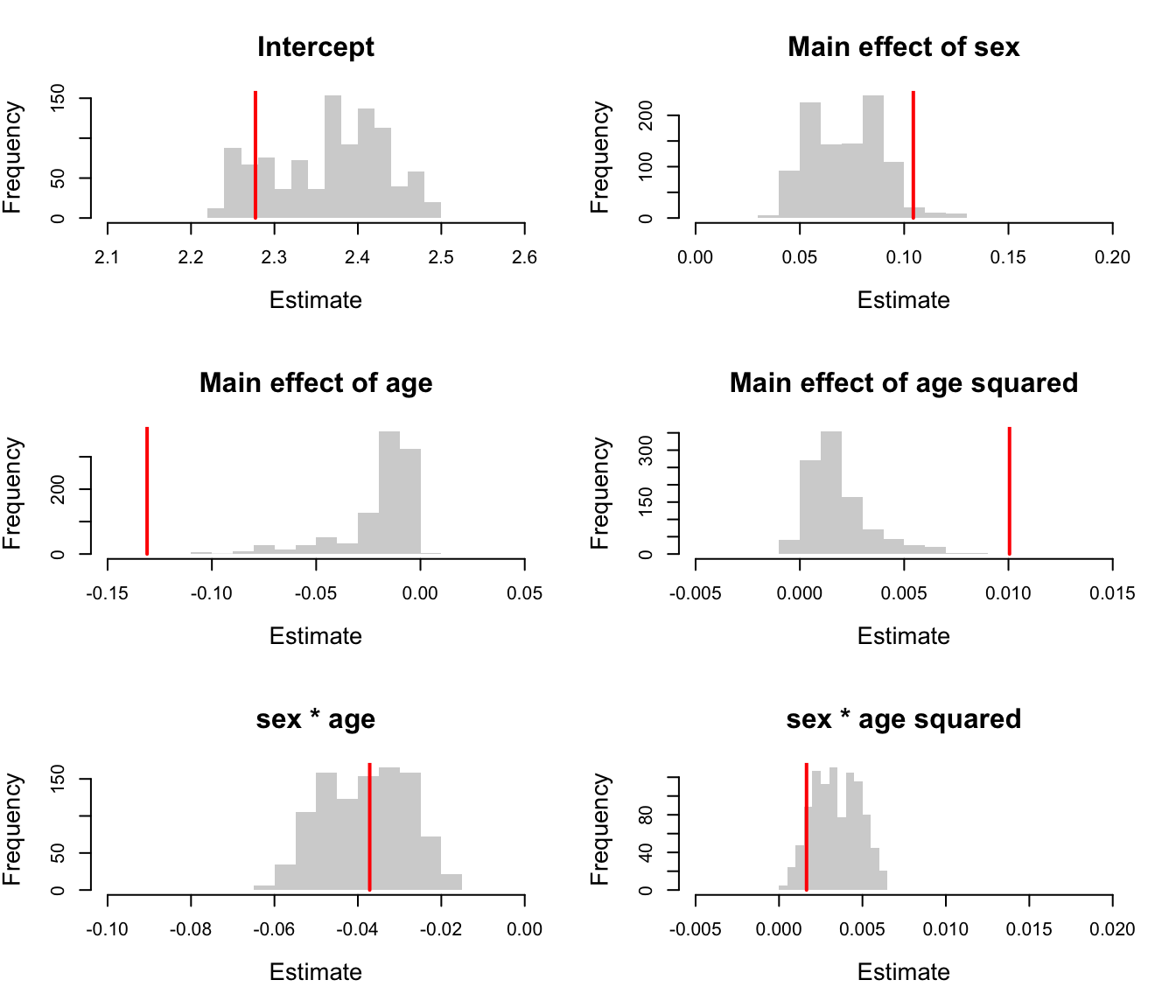
# quantiles of reference distribution
quantile(fixefs[,1],c(0.025,0.975))
#>     2.5%    97.5%
#> 2.245197 2.478587
quantile(fixefs[,2],c(0.025,0.975))
#>       2.5%      97.5%
#> 0.04420932 0.10535789
quantile(fixefs[,3],c(0.025,0.975))
#>         2.5%        97.5%
#> -0.077605512 -0.002002808
quantile(fixefs[,4],c(0.025,0.975))
#>         2.5%        97.5%
#> -0.000169437  0.006084938
quantile(fixefs[,5],c(0.025,0.975))
#>        2.5%       97.5%
#> -0.05608891 -0.02012636
quantile(fixefs[,6],c(0.025,0.975))
#>         2.5%        97.5%
#> 0.0009240526 0.0058891721

# p values
sum(summary(mod_deg2alt)$coefficients$cond[,1][1]<fixefs[,1])/(n.rand+1)
#> [1] 0.8481518
sum(summary(mod_deg2alt)$coefficients$cond[,1][2]<fixefs[,2])/(n.rand+1)
#> [1] 0.02697303
sum(summary(mod_deg2alt)$coefficients$cond[,1][3]<fixefs[,3])/(n.rand+1)
#> [1] 0.999001
sum(summary(mod_deg2alt)$coefficients$cond[,1][4]<fixefs[,4])/(n.rand+1)
#> [1] 0
sum(summary(mod_deg2alt)$coefficients$cond[,1][5]<fixefs[,5])/(n.rand+1)
#> [1] 0.5004995
sum(summary(mod_deg2alt)$coefficients$cond[,1][6]<fixefs[,6])/(n.rand+1)
#> [1] 0.8981019
# plot of fixed effects
par(mfrow=c(3,2))
hist(fixefs[,1],col="light grey",border=NA,xlim=c(2.1,2.6),main="Intercept",xlab="Estimate",cex.lab=1.3,cex.main=1.5)
lines(x=rep(fixef(mod_deg2alt)[[1]][1],2),y=c(0,1000),lwd=2,col="red")
hist(fixefs[,2],col="light grey",border=NA,xlim=c(0,0.2),main="Main effect of sex",xlab="Estimate",cex.lab=1.3,cex.main=1.5)
lines(x=rep(fixef(mod_deg2alt)[[1]][2],2),y=c(0,1000),lwd=2,col="red")
hist(fixefs[,3],col="light grey",border=NA,xlim=c(-0.15,0.05),main="Main effect of age",xlab="Estimate",cex.lab=1.3,cex.main=1.5)
lines(x=rep(fixef(mod_deg2alt)[[1]][3],2),y=c(0,1000),lwd=2,col="red")
hist(fixefs[,4],col="light grey",border=NA,xlim=c(-0.005,0.015),main="Main effect of age squared",xlab="Estimate",cex.lab=1.3,cex.main=1.5)
lines(x=rep(fixef(mod_deg2alt)[[1]][4],2),y=c(0,1000),lwd=2,col="red")
hist(fixefs[,5],col="light grey",border=NA,xlim=c(-0.1,0),main="sex * age",xlab="Estimate",cex.lab=1.3,cex.main=1.5)
lines(x=rep(fixef(mod_deg2alt)[[1]][5],2),y=c(0,1000),lwd=2,col="red")
hist(fixefs[,6],col="light grey",border=NA,xlim=c(-0.005,0.02),main="sex * age squared",xlab="Estimate",cex.lab=1.3,cex.main=1.5)
lines(x=rep(fixef(mod_deg2alt)[[1]][6],2),y=c(0,1000),lwd=2,col="red")
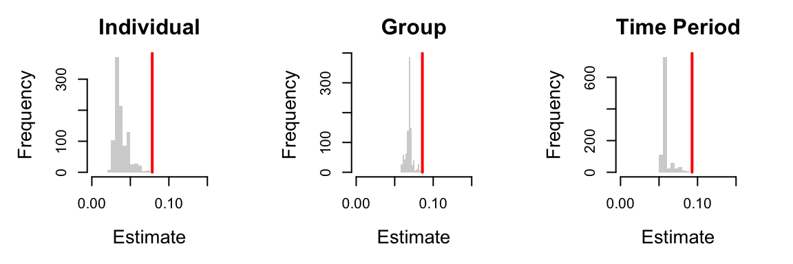
# plot of random effects
par(mfrow=c(1,3),mar=c(5,5,3,3))
hist(ranefs[,1],col="light grey",border=NA,xlim=c(0,0.15),main="Individual",xlab="Estimate",cex.lab=1.3,cex.main=1.5)
lines(x=rep(unlist(summary(mod_deg2alt)[9]$varcor)[1],2),y=c(0,1000),lwd=2,col="red")
hist(ranefs[,2],col="light grey",border=NA,xlim=c(0,0.15),main="Group",xlab="Estimate",cex.lab=1.3,cex.main=1.5)
lines(x=rep(unlist(summary(mod_deg2alt)[9]$varcor)[2],2),y=c(0,1000),lwd=2,col="red")
hist(ranefs[,3],col="light grey",border=NA,xlim=c(0,0.15),main="Time Period",xlab="Estimate",cex.lab=1.3,cex.main=1.5)
lines(x=rep(unlist(summary(mod_deg2alt)[9]$varcor)[3],2),y=c(0,1000),lwd=2,col="red")
# plot of predicted change in degree with age
par(mfrow=c(1,1),mar=c(5,5,3,3))
x<-seq(0,14,0.01)
yf<-unlist(fixef(mod_deg2alt))[1]+unlist(fixef(mod_deg2alt))[3]*x+unlist(fixef(mod_deg2alt))[4]*x^2
ym<-unlist(fixef(mod_deg2alt))[1]+unlist(fixef(mod_deg2alt))[2]+(unlist(fixef(mod_deg2alt))[3]+unlist(fixef(mod_deg2alt))[5])*x+(unlist(fixef(mod_deg2alt))[4]+unlist(fixef(mod_deg2alt))[6])*x^2
plot(x,exp(yf)+1,col="dodger blue",type="l",lwd=4,ylab="Predicted Degree",xlab="Age",cex.lab=1.5,cex.axis=1.3,las=1,ylim=c(5,15))
lines(x,exp(ym)+1,col="firebrick",lwd=4)

for(i in 1:50){
  yf<-fixefs[i,1]+fixefs[i,3]*x+fixefs[i,4]*x^2
  ym<-fixefs[i,1]+fixefs[i,2]+(fixefs[i,3]+fixefs[i,5])*x+(fixefs[i,4]+fixefs[i,6])*x^2
  lines(x,exp(yf)+1,col=adjustcolor("dodgerblue",0.05))
  lines(x,exp(ym)+1,col=adjustcolor("firebrick",0.05))
}
References
- Delahay, R. J., Walker, N., Smith, G. S., Wilkinson, D., Clifton-Hadley, R. S., Cheeseman, C. L., … Chambers, M. A. (2013). Long-term temporal trends and estimated transmission rates for Mycobacterium bovis infection in an undisturbed high-density badger (Meles meles) population. Epidemiology and Infection, 141(07), 1445–1456.
- McDonald, J. L., Robertson, A., & Silk, M. J. (2018). Wildlife disease ecology from the individual to the population: Insights from a long-term study of a naturally infected European badger population. Journal of Animal Ecology, 87(1). doi:10.1111/1365-2656.12743
- Weber, N., Carter, S. P., Dall, S. R. X., Delahay, R. J., McDonald, J. L., Bearhop, S., & McDonald, R. A. (2013). Badger social networks correlate with tuberculosis infection. Current Biology, 23(20), R915–R916.