CMRnet
Matthew Silk
2020-07-03
CMRnet.RmdAn introduction on how to use CMRnet to create, analyse and plot networks from capture, mark, recapture data
# load packages
library(CMRnet)
CMRnet comes with three example datasets loaded which help demonstrate how data should be organised when using CMRnet and how the functions work. In this vignette we will use these example dataset to demonstrate the functions of CMRnet.
# load in data
data(cmrData)
data(cmrData2)
data(cmrData3)

# look at the datasets
str(cmrData)
#> 'data.frame':    1230 obs. of  5 variables:
#>  $ id  : num  69 60 24 26 71 43 17 70 10 79 ...
#>  $ loc : chr  "h" "h" "r" "m" ...
#>  $ x   : num  13 13 20 14 15 14 8 18 18 20 ...
#>  $ y   : num  8 8 2 10 17 10 14 8 3 2 ...
#>  $ date: chr  "2010-01-20" "2010-01-20" "2010-01-20" "2010-01-20" ...
str(cmrData2)
#> 'data.frame':    1230 obs. of  6 variables:
#>  $ id   : num  69 60 24 26 71 43 17 70 10 79 ...
#>  $ loc  : chr  "h" "h" "r" "m" ...
#>  $ x    : num  13 13 20 14 15 14 8 18 18 20 ...
#>  $ y    : num  8 8 2 10 17 10 14 8 3 2 ...
#>  $ date : chr  "2010-01-20" "2010-01-20" "2010-01-20" "2010-01-20" ...
#>  $ layer: Factor w/ 2 levels "F","M": 1 2 2 2 1 1 1 2 2 1 ...
str(cmrData3)
#> 'data.frame':    1191 obs. of  5 variables:
#>  $ id  : int  11 3 18 15 20 23 29 26 3 20 ...
#>  $ loc : Factor w/ 20 levels "a","b","c","d",..: 7 12 14 16 2 6 14 5 16 2 ...
#>  $ x   : int  20 2 7 18 11 12 7 15 18 11 ...
#>  $ y   : int  10 9 5 18 13 8 5 14 18 13 ...
#>  $ date: POSIXct, format: "2020-06-18 02:32:01" "2020-06-18 02:32:01" ...
1. Creating networks from mark-recpature data
A principal aim of the package is to facilitate the construction of networks from mark-recapture data. CMRnet can be used to construct two types of social network:
- Co-capture (social) networks. These networks connect two individuals that have been captured at the same location (or close by) within a pre-defined time interval
- Movement networks. These networks connect two locations that an individual has been trapped at with a directed edge. CMRnet enables movement networks to be constructed as multiplex networks in which different layers represent the movements of different types of individual (female vs. male, different age classes etc.)
In both co-capture and movement networks, the package allows the use of either date or date/time information to construct social networks. The former will be applicable to most types of mark-recapture data, but the latter will be useful when capture events occur at much higher resolutions.
First we construct co-capture networks using the the normal and high resolution versions of the co-capture network function. The normal version DynamicNetCreate() defines the interval window in days.
# Set parameters for the function ####

# Start Date
mindate <- "2010-01-01"
# End Date
maxdate <- "2015-01-01"
# Length of time in days within which individuals are considered to be co-captured
intwindow <- 60
# Length of each network window in months. We will use 5 12-month windows in this example
netwindow <- 12
# Overlap between network windows in months (we have no overlap in this example)
overlap <- 0
# Spatial tolerance for defining co-captures. Captures within a threshold distance (rather than simply at the same location) are considered when this is set to be greater than zero
spacewindow <- 0

# Create co-capture (social) networks ####
# index=FALSE indicates that we want edges to be weighted by the number of movements (see help pages for the alternative)
netdat <- DynamicNetCreate(
    data = cmrData,
    intwindow = intwindow,
    mindate = mindate,
    maxdate = maxdate,
    netwindow = netwindow,
    overlap = overlap,
    spacewindow = spacewindow,
    index=FALSE
  )
#> [1] "End of final network window aligns with end of study"
[==================================================================] 100%
[==================================================================] 100%
[==================================================================] 100%
[==================================================================] 100%
[==================================================================] 100%
The high resolution DynamicNetCreateHi sets the interval window in minutes.
# Set parameters for the function ####
mindate <- "2019-12-01 00:00:00"
maxdate <- "2020-07-01 00:00:00"
# The interaction window is now in minutes. We set it to be one day here.
intwindow <- 24*60
# The network window is now in days
netwindow <- 20
# The overlap is now also in days
overlap <- 2
spacewindow <- 0

## Create high-resolution co-capture (social) networks
netdat_hi<-DynamicNetCreateHi(
  data=cmrData3,
  intwindow=intwindow,
  mindate=mindate,
  maxdate=maxdate,
  netwindow=netwindow,
  overlap=overlap,
  spacewindow=spacewindow,
  index=FALSE)
#> [1] "Final network window stops 18720 minutes before the end of the study"
[==================================================================] 100%
[==================================================================] 100%
[==================================================================] 100%
[==================================================================] 100%
[==================================================================] 100%
[==================================================================] 100%
[==================================================================] 100%
[==================================================================] 100%
[==================================================================] 100%
[==================================================================] 100%
[==================================================================] 100%
Next we do the same for the creation of single layer movement networks using MoveNetCreate and MoveNetCreateHi.
# Set parameters for the function ####

#Start Date
mindate <- "2010-01-01"
# End Date
maxdate <- "2015-01-01"
# Length of time in days within which individuals are considered to be co-captured
intwindow <- 60
# Length of each network window in months. We will use 5 12-month windows in this example
netwindow <- 12
# Overlap between network windows in months (we have no overlap in this example)
overlap <- 0

# Generate movement network
# nextonly=TRUE indicates that only direct movements between groups should be considered (see help pages)
movenetdat <- MoveNetCreate(
  data = cmrData,
  intwindow = intwindow,
  mindate = mindate,
  maxdate = maxdate,
  netwindow = netwindow,
  overlap = overlap,
  nextonly = TRUE,
  index=FALSE
)
#> [1] "End of final network window aligns with end of study"
[==================================================================] 100%
[==================================================================] 100%
[==================================================================] 100%
Again the high resolution MoveNetCreateHi defines the interval window in minutes.
# Set parameters for the function ####
mindate <- "2019-12-01 00:00:00"
maxdate <- "2020-07-01 00:00:00"
# Interaction window is now in minutes
intwindow <- 30*24*60
# The network window is now in days
netwindow <- 60
#The overlap is now also in days
overlap <- 0
spacewindow <- 0

# Generate movement network
# nextonly=TRUE indicates that only direct movements between groups should be considered (see help pages)
movenetdat_hi <- CMRnet::MoveNetCreateHi(
  data = cmrData3,
  intwindow = intwindow,
  mindate = mindate,
  maxdate = maxdate,
  netwindow = netwindow,
  overlap = overlap,
  nextonly = TRUE,
  index=FALSE
)
#> [1] "Final network window stops 1567049760 minutes before the end of the study"
[==================================================================] 100%
[==================================================================] 100%
[==================================================================] 100%
Next we construct multiplex movement networks using the standard function to show how to use the alternative data format. These networks are useful when there are multiple layered movement networks (i.e. a separate network for males and females).
#Start Date
mindate <- "2010-01-01"
# End Date
maxdate <- "2015-01-01"
# Length of time in days within which individuals are considered to be co-captured
intwindow <- 60
# Length of each network window in months. We will use 5 12-month windows in this example
netwindow <- 12
# Overlap between network windows in months (we have no overlap in this example)
overlap <- 0

# Generate multiplex movement network
multimovenetdat <-
  CMRnet::MultiMoveNetCreate(
    data = cmrData2,
    intwindow = intwindow,
    mindate = mindate,
    maxdate = maxdate,
    netwindow = netwindow,
    overlap = overlap,
    nextonly = TRUE,
    index=FALSE
  )
#> [1] "End of final network window aligns with end of study"
2. Conversion to igraph objects and plotting
Above we have demonstrated how to generate networks using CMRnet. Next we demonstrate the package’s functionality for onward analysis and plotting.
To facilitate analysis we provide a function that can convert CMRnet objects into lists of igraph objects. This is a commonly-used network analysis package in R that provides various functions to calculate individual and network-level measures of network structure.
We also provide functions that can produce plots of these lists of igraph networks to enable basic visualisation of the networks produced.
Here is an example where plot a social network.
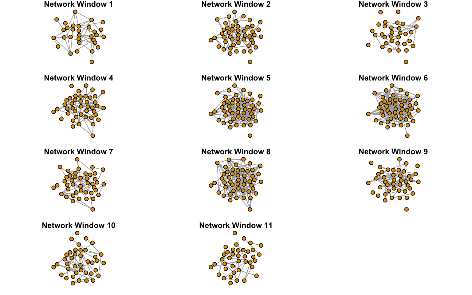
##Convert social networks into a list of igraph networks
cc_nets<-CMRnet::cmr_igraph(netdat_hi,type="social")

#Look at the structure of the object generated
print(cc_nets)
#> [[1]]
#> [[1]][[1]]
#> IGRAPH 7d093cc UNW- 31 34 --
#> + attr: name (v/c), weight (e/n)
#> + edges from 7d093cc (vertex names):
#>  [1] 4 --22 4 --23 5 --42 6 --23 6 --25 6 --30 6 --43 6 --50 9 --28 9 --29
#> [11] 9 --42 10--49 16--19 21--23 22--31 22--40 22--43 22--49 23--25 23--50
#> [21] 25--41 25--50 27--50 28--29 28--42 29--42 30--31 30--32 30--43 31--32
#> [31] 31--43 31--49 43--46 43--49
#>
#> [[1]][[2]]
#> IGRAPH d4a17f8 UNW- 48 65 --
#> + attr: name (v/c), weight (e/n)
#> + edges from d4a17f8 (vertex names):
#>  [1] 2 --36 3 --4  3 --19 3 --40 4 --22 6 --11 6 --23 6 --25 6 --29 6 --30
#> [11] 6 --38 6 --43 6 --50 7 --10 7 --16 7 --32 9 --13 9 --26 9 --28 9 --42
#> [21] 10--32 10--37 10--49 11--29 11--46 12--17 13--20 13--26 13--44 13--50
#> [31] 14--43 16--19 16--36 17--25 17--32 17--37 18--27 19--24 19--35 20--21
#> [41] 20--22 20--24 20--39 20--44 21--39 22--23 22--24 22--36 22--42 23--25
#> [51] 23--36 23--50 24--35 25--32 25--50 26--38 27--31 27--33 27--50 28--42
#> [61] 30--43 31--33 34--42 37--49 47--50
#>
#> [[1]][[3]]
#> IGRAPH 0c7a5e0 UNW- 33 27 --
#> + attr: name (v/c), weight (e/n)
#> + edges from 0c7a5e0 (vertex names):
#>  [1] 1 --28 2 --38 2 --40 3 --11 3 --46 6 --22 6 --26 6 --38 8 --27 9 --13
#> [11] 10--34 11--46 12--18 12--34 12--36 13--37 18--34 18--36 22--26 22--34
#> [21] 22--38 24--26 26--38 34--36 35--36 38--40 48--50
#>
#> [[1]][[4]]
#> IGRAPH bcf1961 UNW- 43 65 --
#> + attr: name (v/c), weight (e/n)
#> + edges from bcf1961 (vertex names):
#>  [1] 1 --6  1 --34 1 --47 1 --49 2 --13 2 --35 3 --11 3 --24 3 --39 3 --46
#> [11] 4 --40 4 --47 5 --29 5 --36 5 --42 5 --44 6 --34 6 --49 8 --20 8 --22
#> [21] 8 --43 9 --31 10--12 10--35 10--45 10--50 11--23 11--24 11--32 11--46
#> [31] 11--49 12--35 12--45 12--50 13--19 13--35 13--47 13--50 14--19 14--25
#> [41] 14--33 15--20 15--47 19--20 19--33 19--35 19--47 19--50 20--39 20--47
#> [51] 22--43 22--49 23--49 26--31 29--42 29--43 29--44 33--47 34--49 35--45
#> [61] 35--50 40--47 42--44 42--48 45--50
#>
#> [[1]][[5]]
#> IGRAPH c76c0fc UNW- 50 150 --
#> + attr: name (v/c), weight (e/n)
#> + edges from c76c0fc (vertex names):
#>  [1] 1 --2  1 --13 1 --43 1 --45 1 --49 2 --11 2 --18 2 --20 2 --27 2 --33
#> [11] 2 --39 2 --40 2 --42 2 --48 3 --11 3 --24 3 --44 4 --25 4 --27 4 --28
#> [21] 4 --33 4 --43 6 --20 7 --16 7 --44 8 --13 8 --20 8 --22 8 --34 8 --43
#> [31] 9 --40 10--20 10--40 10--41 10--50 11--19 11--22 11--24 11--27 11--28
#> [41] 11--32 12--14 12--34 13--14 13--24 13--27 13--29 13--36 13--37 13--39
#> [51] 13--42 13--45 13--47 14--15 14--17 14--27 14--34 14--36 14--37 14--42
#> [61] 15--17 15--21 15--35 15--38 16--30 16--44 17--23 17--27 17--28 17--47
#> [71] 17--48 18--23 18--49 19--20 19--21 19--22 19--24 19--32 19--33 19--35
#> + ... omitted several edges
#>
#> [[1]][[6]]
#> IGRAPH c3cdfc8 UNW- 49 177 --
#> + attr: name (v/c), weight (e/n)
#> + edges from c3cdfc8 (vertex names):
#>  [1] 1 --7  1 --14 1 --18 1 --24 1 --28 1 --30 1 --33 1 --35 1 --43 1 --44
#> [11] 1 --45 1 --50 2 --37 2 --41 3 --12 3 --13 3 --15 3 --26 3 --27 3 --32
#> [21] 3 --37 3 --50 4 --6  4 --9  4 --10 4 --31 5 --34 6 --7  6 --10 6 --31
#> [31] 6 --47 7 --35 7 --47 7 --50 8 --29 9 --14 9 --16 9 --18 9 --19 9 --20
#> [41] 9 --33 9 --34 10--19 10--31 10--32 10--34 10--36 11--22 11--35 11--45
#> [51] 11--47 11--48 12--31 12--32 12--33 12--35 12--36 12--45 12--48 13--15
#> [61] 13--18 13--26 13--27 13--37 14--16 14--20 14--30 14--33 14--35 14--47
#> [71] 15--20 15--26 15--27 15--37 15--47 16--20 16--33 16--39 16--43 16--47
#> + ... omitted several edges
#>
#> [[1]][[7]]
#> IGRAPH 5e6d19d UNW- 43 52 --
#> + attr: name (v/c), weight (e/n)
#> + edges from 5e6d19d (vertex names):
#>  [1] 1 --11 1 --21 2 --20 3 --5  3 --36 3 --41 4 --31 4 --46 5 --36 5 --41
#> [11] 6 --32 8 --47 9 --35 11--19 11--21 11--26 11--29 11--48 12--17 12--23
#> [21] 12--48 16--19 16--20 17--23 18--32 18--40 19--20 19--26 19--29 19--48
#> [31] 20--26 20--41 24--32 24--50 26--29 26--30 26--37 26--41 26--44 26--48
#> [41] 27--40 27--49 29--48 30--37 30--44 31--46 32--33 32--50 36--41 37--44
#> [51] 40--49 41--48
#>
#> [[1]][[8]]
#> IGRAPH 29b7e48 UNW- 49 162 --
#> + attr: name (v/c), weight (e/n)
#> + edges from 29b7e48 (vertex names):
#>  [1] 1 --3  1 --6  1 --10 1 --12 1 --13 1 --18 1 --21 1 --26 1 --32 1 --42
#> [11] 1 --43 2 --3  2 --8  2 --12 2 --13 2 --20 2 --24 2 --37 2 --40 3 --12
#> [21] 3 --13 3 --20 3 --26 3 --31 3 --37 3 --43 3 --46 4 --5  4 --9  4 --12
#> [31] 4 --20 4 --22 4 --27 4 --36 4 --39 5 --12 5 --24 5 --27 5 --48 6 --13
#> [41] 6 --18 6 --26 6 --31 6 --32 6 --34 6 --43 7 --16 7 --17 7 --20 7 --21
#> [51] 7 --26 7 --28 7 --34 7 --39 7 --44 7 --48 7 --49 8 --12 8 --17 8 --32
#> [61] 8 --37 8 --42 8 --43 9 --26 9 --27 9 --34 9 --38 9 --39 9 --46 10--13
#> [71] 10--21 10--32 10--37 11--42 11--50 12--14 12--17 12--22 12--23 12--26
#> + ... omitted several edges
#>
#> [[1]][[9]]
#> IGRAPH 3131c34 UNW- 43 58 --
#> + attr: name (v/c), weight (e/n)
#> + edges from 3131c34 (vertex names):
#>  [1] 1 --3  1 --25 1 --27 1 --36 1 --38 1 --39 2 --4  2 --10 2 --31 2 --34
#> [11] 3 --11 3 --24 3 --28 3 --38 3 --39 3 --49 4 --10 6 --21 6 --25 8 --10
#> [21] 8 --11 8 --19 8 --40 9 --10 9 --21 9 --22 9 --29 9 --34 9 --35 9 --47
#> [31] 10--11 10--19 10--23 10--26 10--47 10--48 11--28 11--38 12--35 12--45
#> [41] 14--28 14--38 19--29 22--29 22--34 22--35 26--48 27--36 28--32 28--38
#> [51] 28--49 29--34 29--35 31--32 31--34 34--35 35--45 38--47
#>
#> [[1]][[10]]
#> IGRAPH 52aa49d UNW- 39 40 --
#> + attr: name (v/c), weight (e/n)
#> + edges from 52aa49d (vertex names):
#>  [1] 1 --7  1 --38 2 --33 6 --13 6 --14 6 --35 6 --38 6 --40 6 --47 8 --40
#> [11] 12--26 12--36 12--50 13--35 14--17 14--25 14--32 14--42 14--47 14--48
#> [21] 18--23 19--29 23--48 25--32 25--42 25--48 26--29 26--43 26--48 28--41
#> [31] 29--36 29--43 31--50 32--42 32--48 35--37 38--39 38--40 42--48 43--49
#>
#> [[1]][[11]]
#> IGRAPH 5c5c6dd UNW- 39 32 --
#> + attr: name (v/c), weight (e/n)
#> + edges from 5c5c6dd (vertex names):
#>  [1] 1 --9  1 --33 1 --47 3 --8  3 --17 3 --28 3 --50 4 --11 4 --18 6 --13
#> [11] 6 --35 8 --12 8 --17 9 --47 11--18 12--26 12--50 13--35 15--22 15--43
#> [21] 21--35 21--41 22--43 26--29 26--43 28--47 29--36 29--40 29--43 31--46
#> [31] 35--41 38--39
#>
#>
#> [[2]]
#> IGRAPH 04f3925 UNW- 50 607 --
#> + attr: name (v/c), weight (e/n)
#> + edges from 04f3925 (vertex names):
#>   [1] 1--2  1--3  1--6  1--7  1--9  1--10 1--11 1--12 1--13 1--14 1--18 1--21
#>  [13] 1--24 1--25 1--26 1--27 1--28 1--30 1--32 1--33 1--34 1--35 1--36 1--38
#>  [25] 1--39 1--42 1--43 1--44 1--45 1--47 1--49 1--50 2--3  2--4  2--8  2--10
#>  [37] 2--11 2--12 2--13 2--18 2--20 2--24 2--27 2--31 2--33 2--34 2--35 2--36
#>  [49] 2--37 2--38 2--39 2--40 2--41 2--42 2--48 3--4  3--5  3--8  3--11 3--12
#>  [61] 3--13 3--15 3--17 3--19 3--20 3--24 3--26 3--27 3--28 3--31 3--32 3--36
#>  [73] 3--37 3--38 3--39 3--40 3--41 3--43 3--44 3--46 3--49 3--50 4--5  4--6
#>  [85] 4--9  4--10 4--11 4--12 4--18 4--20 4--22 4--23 4--25 4--27 4--28 4--31
#> + ... omitted several edges
#Note that cc_nets[[1]] is a list of the networks for each network window and cc_nets[[2]] is the overall (aggregated) network

##Now we can plot the networks produced
#Setting fixed_locs to TRUE means nodes have the same coordinates in each plot
#Setting dynamic to FALSE and rows to 2 means we produce a multipanelled figure with 2 rows
#We can use additional arguments from the plot.igraph function. Here we suppress node labels as an example.
CMRnet::cmrSocPlot(nets=cc_nets,fixed_locs=TRUE,dynamic=FALSE,rows=4,vertex.label=NA)
And here is an example where plot a movement network.
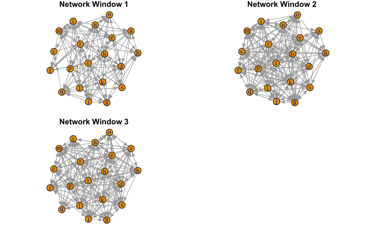
##Convert social networks into a list of igraph networks
m_nets<-CMRnet::cmr_igraph(movenetdat_hi,type="movement")

##Now we can plot the networks produced
#Setting fixed_locs to TRUE means nodes have the same coordinates in each plot
#Setting dynamic to FALSE and rows to 2 means we produce a multipanelled figure with 2 rows
#We can use additional arguments from the plot.igraph function. Here we suppress node labels as an example.
CMRnet::cmrMovPlot(nets=m_nets,fixed_locs=TRUE,dynamic=FALSE,rows=2,edge.arrow.size=0.5)
The cmr_igraph function can be used in much the same way for multiplex network objects, but the plotting is rather different using a 3d scatterplot to show the layers together.
##Convert social networks into a list of igraph networks
mm_nets<-CMRnet::cmr_igraph(multimovenetdat,type="multiplex")

##Now we can plot the networks produced
#Setting fixed_locs to TRUE means nodes have the same coordinates in each plot
#Setting dynamic to FALSE and rows to 2 means we produce a multipanelled figure with 2 rows
#We can use additional arguments from the plot.igraph function. Here we suppress node labels as an example.
CMRnet::cmrMultiplexPlot(nets=mm_nets,fixed_locs=TRUE,dynamic=FALSE,rows=2,layer_colours=c("dodgerblue","firebrick"))
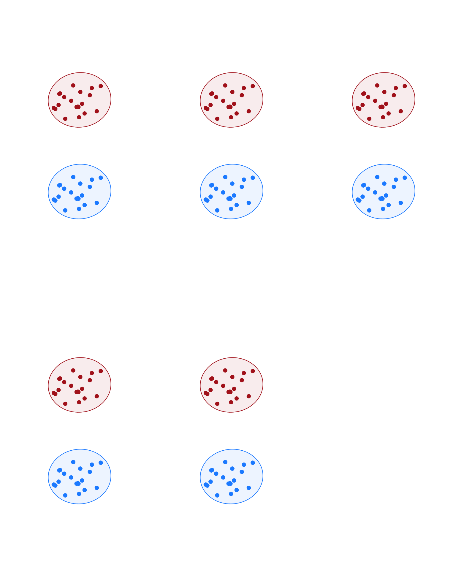
NOTE: The functionality for plotting multiplex networks in this way is rather limited and intended to provide basic visualisations. If more sophisticated plots are required then the function can be adjusted by the user to suit their preferences
3. Permutation approaches in CMRnet
We now demonstrate how CMRnet can be used to conduct permutations of networks generated using the package. These permutations can be used for statistical inference.
Two broad types of permutations are possible within CMRnet.
- Post-network permutations are node swaps that result in different node IDs being shuffled around the network. These permutations break the correlation between particular node traits and network properties and so are excellent for testing hypotheses focussed on the association between particular traits and social network measures. For example, if a reasearcher hypothesises that females have higher degree (more connections) in a network than males, then post-network permutations randomise the network with respect to this relationship and so provide an excellent reference model to test whether it is different to that expected by chance.
- Pre-network or datastream permutations shuffle the raw capture data, swapping the identity of individual captured (for co-capture/social networks) or the location of the capture (for movement networks) between different capture events. These types of permutations provide an excellent tool for assessing whether a network is different to random within the particular set of constraints imposed by the permutation, and can control for sampling effects (e.g. some individuals being captured more often or more captures occurring at particular locations).
Post-network permutations can be conducted in two ways in CMRnet. Unrestricted swaps are conducted using the function cmrNodeswap() which is demonstrated here. Swaps can also be restricted to only occur between particular pairs of individuals (e.g. those captured at the same locations) and are demonstrated in one of the empirical case studies.
##Unrestricted node swaps
#Note that you can set the desired number of permuted networks and need to indicate whether the network is multiplex or not
ns_nets <- CMRnet::cmrNodeswap(netdat, n.rand = 1000, multi = FALSE)

#Show dimensions of output object
lapply(ns_nets,dim)
#> [[1]]
#> [1]  180  180 1000
#>
#> [[2]]
#> [1]  180  180 1000
#>
#> [[3]]
#> [1]  180  180 1000
#>
#> [[4]]
#> [1]  180  180 1000
#>
#> [[5]]
#> [1]  180  180 1000
The output of the post-network permutations is a list, where each element of the list corresponds to a particular network window and contains an array of the permuted networks for that window. For multiplex networks this list is nested (see manual pages).
Pre-network permutations have separate functions for co-capture (social) networks and movement networks and we demonstrate both below. They differ through the DatastreamPermSoc() function swapping individual identities between capture events and the DatastreamPermSpat() function swapping locations instead.
First we will permute co-capture networks.
## Reset parameters for co-capture network generation
mindate <- "2010-01-01"
maxdate <- "2015-01-01"
intwindow <- 60
netwindow <- 12
overlap <- 0
spacewindow <- 0

## Set new parameter for the permutations
#Whether swaps should be constrained to occur only between capture events at the same time
same.time = FALSE
#An upper limit for the number of days between capture events for swaps to be allowed
time.restrict = 6
#Whether swaps should be constrained to occur only between capture events at the same location
same.spat = FALSE
#Whether swaps should be constrained to occur within a threshold distance (setting to "n" means this argument is ignored)
spat.restrict = "n"
#The length of the burn-in period before networks are saved
n.burnin = 10
#The number  of swaps between each saved result
n.swaps = 5
#The number of permuted datasets to be saved. Not we have set this to be small so that the function runs quickly (normally it would be 1000, 10,000 etc.)
n.rand = 2
#The number of days around a capture event that an individual can't be swapped into (see manual pages)
buffer = 0

## Run permutations
#Note we have set iter=FALSE here. iter=TRUE allows these swaps to be conducted one at a time to help with memory issues
Rs <- CMRnet::DatastreamPermSoc(
    data = cmrData,
    intwindow,
    mindate,
    maxdate,
    netwindow,
    overlap,
    spacewindow,
    same.time,
    time.restrict,
    same.spat,
    spat.restrict,
    n.swaps,
    n.rand,
    burnin = TRUE,
    n.burnin,
    iter = FALSE,
    buffer=buffer
  )
#> [1] "End of final network window aligns with end of study"

#The first element of the output is a list where each element corresponds to a network window and contains an array with the permuted networks.
lapply(Rs[[1]],dim)
#> [[1]]
#> [1] 180 180   2
#>
#> [[2]]
#> [1] 180 180   2
#>
#> [[3]]
#> [1] 180 180   2
#>
#> [[4]]
#> [1] 180 180   2
#>
#> [[5]]
#> [1] 180 180   2

#The second element is the new node.exist indicator
dim(Rs[[2]])
#> [1] 180   6

##If instead we set iter=TRUE
#(not we have changed some of the other arguments too)
Rs2 <- CMRnet::DatastreamPermSoc(
    data = cmrData,
    intwindow,
    mindate,
    maxdate,
    netwindow,
    overlap,
    spacewindow,
    same.time,
    time.restrict,
    same.spat,
    spat.restrict,
    n.swaps=10,
    n.rand=1,
    burnin = FALSE,
    n.burnin=0,
    iter = TRUE,
    buffer=buffer
  )
#> [1] "End of final network window aligns with end of study"

#Instead, Rs2[[1]] is the new dataframe after the swaps, Rs2[[2]] are the networks and Rs2[[3]] the new node.exist
dim(Rs2[[1]])
#> [1] 1230    5
Now movement networks.
## Reset parameters for co-capture network generation
mindate <- "2010-01-01"
maxdate <- "2015-01-01"
intwindow <- 60
netwindow <- 12
overlap <- 0

same.time=FALSE
time.restrict=6
spat.restrict="n"
#Whether to restrict swaps by the identity of the individual captured
same.id=FALSE
n.swaps=10
n.rand=100
n.burnin=100
warn.thresh=10000

mRs <- CMRnet::DatastreamPermSpat(
  data = cmrData,
  intwindow=intwindow,
  mindate=mindate,
  maxdate=maxdate,
  netwindow=netwindow,
  overlap=overlap,
  nextonly = TRUE,
  same.time=same.time,
  time.restrict=time.restrict,
  spat.restrict=spat.restrict,
  same.id=same.id,
  n.swaps=n.swaps,
  n.rand=n.rand,
  burnin = TRUE,
  n.burnin=n.burnin,
  warn.thresh=warn.thresh,
  iter = FALSE
)
#> [1] "End of final network window aligns with end of study"

#Demonstrate that the randomised networks have been saved correctly
lapply(mRs[[1]],dim)
#> [[1]]
#> [1]  20  20 100
#>
#> [[2]]
#> [1]  20  20 100
#>
#> [[3]]
#> [1]  20  20 100
#>
#> [[4]]
#> [1]  20  20 100
#>
#> [[5]]
#> [1]  20  20 100